All the Truth about Static Analysis

Recently, we have increasingly heard about the importance of static analysis as a tool for newly developed software quality assurance, especially in terms of security. Static analysis helps discover vulnerabilities and other errors and can be integrated into existing processes and thus used during development. However, this raises many questions. What is the difference between free and commercial tools? Why using a linter is not enough? And what do statistics have to do with it? Let’s see. 

We’ll answer the last question first: although static analysis is often wrongly called statistical, in reality statistics have nothing to do with it. The analysis is in fact static, since an application is not running while being scanned. 

First, let’s figure out what to look for in a program code. Static analysis is most often employed to reveal vulnerabilities, i.e. those code fragments that can lead to a confidentiality breach or ruin information system integrity or availability. However, the same technology can be used to search for other errors or code peculiarities. 

In general, the static analysis problem is algorithmically unsolvable as we can see, for example, from Rice’s theorem. Therefore, you have to either limit problem conditions or allow for inaccurate results (e.g. miss vulnerabilities, return false positives). When it comes to real-life programs, the second option is much better. 

Many commercial and free tools claim to search for vulnerabilities in applications written in different programming languages. Let’s examine a typical static analyzer inside and focus on its core and algorithms. Of course, tools differ in terms of user friendliness, functionality, available plugins for third-party systems, and API ease of use. Perhaps, a separate post can be written to cover this topic.

Intermediate representation

The static analyzer operation sequence includes three main steps:

1.    Building an intermediate representation (also called an internal representation or code model)

2.    Using static analysis algorithms to augment the code model with new information

3.    Applying vulnerability search rules to the augmented code model

Different static analyzers may use different code models, such as a source code, token stream, parse tree, three-address code, control flow graph, bytecode (standard or native), etc.

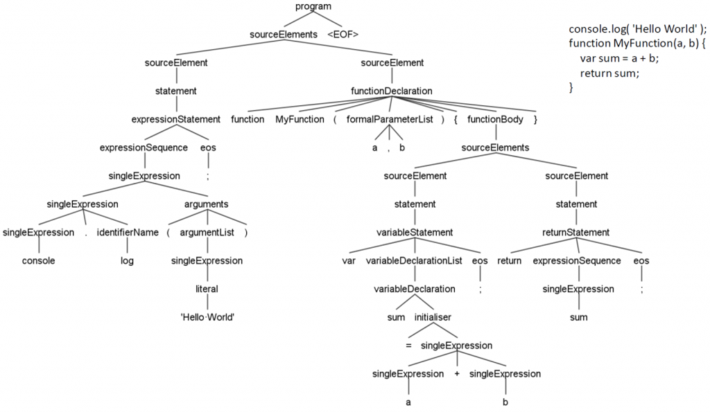
Similar to compilers, lexical and syntax analyses are used to build an internal representation, which is most often a parse tree (also called Abstract Syntax Tree, or AST). Lexical analysis breaks a program text into minimum semantic elements and then outputs a token stream. Syntax analysis checks that the token stream matches the programming language grammar, i.e. the resulting token stream is correct in terms of language. Syntax analysis results in a parse tree, i.e. a structure simulating the program source code. Next, semantic analysis is applied to check the fulfillment of more complex conditions (e.g. data type matching in assignment instructions).

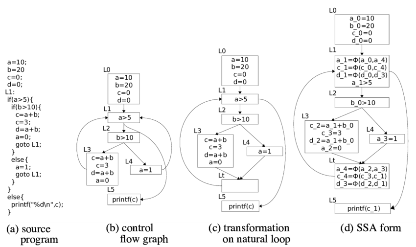
A parse tree can be used either as an internal representation or to build other models. For example, you can translate it into a three-address code, which, in turn, is used to build a control flow graph (CFG). Typically, CFG is a key model for static analysis algorithms.

In case of binary analysis (i.e. static analysis of a binary or executable code), a model is built too, although reverse engineering methods are used such as decompilation, deobfuscation, and reverse translation. As a result, you can obtain the same models as from a source code, including the source code itself (when a full decompilation is used). Sometimes a binary code itself can act as an intermediate representation.

In theory, the closer a model is to the source code, the worse analysis quality is. In a source code itself, you can only search by regular expressions and are therefore limited to discovering just the simplest vulnerabilities.

Dataflow analysis

Dataflow analysis is one of the main static analysis algorithms that has to determine — in each program point — some information about the data handled by the code (e.g. data type or value, etc.). Depending on what information needs to be determined, we can set a dataflow analysis problem.

For example, if we need to check whether an expression is a constant and determine its value, then a constant propagation problem has to be solved. If we need to determine the variable type, then we can talk about a type propagation problem. Or, if we need to understand which variables can point to a specific memory area (store the same data), then this represents an alias analysis problem. There are many other dataflow analysis problems that can be addressed by a static analyzer. Similar to code model building stages, these problems are also solved by compilers. 

Compiler theory offers solutions to an intraprocedural dataflow analysis problem (when data should be tracked within a single procedure/function/method). Such solutions are based on the algebraic lattice theory and other mathematical theory elements. The dataflow analysis problem can be solved in polynomial (i.e. computationally acceptable) time, if the problem setting meets solubility theorem conditions, which is not always the case. 

Let’s discuss solving the intraprocedural dataflow analysis problem in more detail. To set a specific problem, we need to define both the information to be sought and the rules by which this information is modified when data goes through CFG instructions. Keep in mind that CFG nodes are basic blocks, i.e. sets of instructions, which are always executed sequentially, and CFG arcs indicate possible transfers of control between the basic blocks. 

For each instruction S, the following sets are identified:

·         gen(S) (information generated by S),

·         kill(S) (information deleted by S),

·         in(S) (information in point before S),

·         out(S) (information in point after S).

Dataflow analysis aims to identify in(S) and out(S) sets for each instruction S of the program. A basic system of equations used to solve the dataflow analysis problems consists of the following dataflow equations:

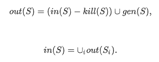
The second equation sets forth the rules to “aggregate” information at CFG arc merge points (Si are S predecessors in CFG). Union, intersection, and some other operations may be used.

The sought information (the value set of the above-introduced functions) is formalized as an algebraic lattice, while the gen and kill functions are treated as monotone mappings on lattices (flow functions). For dataflow equations, the solution is a fixed point of these mappings.

Algorithms for solving dataflow analysis problems look for maximum fixed points. There are several solution approaches: iterative algorithms, strongly connected component analysis, T1-T2 analysis, interval analysis, structural analysis, etc. Theorems on the correctness of these algorithms define the scope of their applicability to real problems. A reminder: theorem conditions may not always be fulfilled, which complicates algorithms and impairs result accuracy.

Interprocedural analysis

In practice, solving interprocedural dataflow analysis problems is often a must-do since vulnerabilities are rarely limited to a single function. There are several general algorithms.

Function inlining: In a function call site, we embed a called function, thus reducing an interprocedural analysis problem to an intraprocedural one. While easy-to-do, in practice, this method quickly causes a combinatorial explosion.

Building a general program CFG where function calls are replaced by transitions to a start address of a respective called function. Return instructions are replaced by transitions to all instructions following all instructions for calling this function. This approach adds a lot of unrealizable execution paths, thus greatly reducing analysis accuracy.

An algorithm is similar to the previous method except that when transiting to a function, the context is saved (for example, a stack frame). This solves the unrealizable path creation problem. However, this algorithm is applicable in case of limited call nesting only.

Building a function summary: This is the most common interprocedural analysis algorithm based on building a summary for each function: the rules regarding which information about data is transformed when applying this function, depending on input argument values. These summaries are used for intraprocedural function analysis. Another challenge here is determining the function traversal sequence since, for intraprocedural analysis, a summary should already be built for all called functions. Usually, special iterative algorithms for call graph traversal are developed.

Interprocedural dataflow analysis is an exponentially complex problem, which is why the analyzer needs to make optimizations and assumptions, since finding an exact solution in a computationally acceptable time is impossible. Usually, when developing an analyzer, we have to find a tradeoff between resource consumption, analysis time, false positive rate and detected vulnerabilities. Therefore, although a static analyzer may be slow, consume a lot of resources and return false positives, you can’t do without one if you want to discover the most critical vulnerabilities.

It is when a good static analyzer prevails over the wide range of free tools claiming to detect vulnerabilities as well. Fast checks in linear time are great when you need to get a result quickly, for example, during compilation. However, this approach cannot find the most critical vulnerabilities, like data injections.

Taint analysis

Another dataflow analysis problem worth noting is taint analysis, which allows for flag propagation across a program. This problem is critical to information security, since it helps detect vulnerabilities related to data injection (SQL injection, cross site scripting, open redirects, file path forging, etc.) and confidential data leaks (such as password writing to event logs, insecure data transfer).

Let’s try to simulate a problem. Suppose we want to track n flags: f1,f2,...,fn. Here, an information set will be a set of subsets {f1,…,fn}, since we want to define flags for each variable in each program point.

Next, we need to define flow functions. In this case, these can be determined via the following considerations.

·         There is a set of rules defining structures that make a flag set appear or change.

·         The assignment operation moves flags from the right to the left.

·         Any operation unknown to rule sets aggregates flags from all operands, and the final flag set is added to the operation results.

Finally, we need to define the rules for merging information in CFG arc merge points. Merging is determined by the union rule, i.e. if different flag sets for one variable came from different basic blocks, they are united when merging. Among other things, this leads to false positives: the algorithm does not guarantee that a CFG path where a flag has occurred can be executed.

Suggest that we need to detect SQL injection. This vulnerability occurs when unverified data from a user enters database handling methods. We must check that data is received from a user and add a taint flag to such data. Typically, an analyzer’s rule base includes taint flag setting rules. For example, set a flag to a value returned by getParameter () method of the Request class.

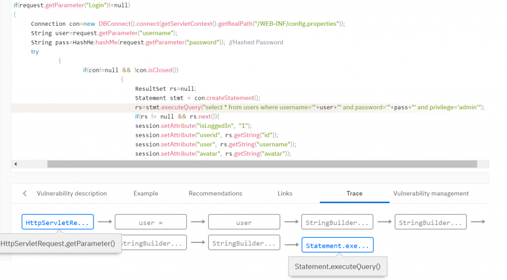
Then, we use taint analysis to propagate the flag throughout the analyzed program, taking into account the fact that data may be validated and the flag may disappear at one of the execution paths. The analyzer has many functions that clear flags. For example, a function validating data from html tags can clear a flag for cross-site scripting (XSS) vulnerabilities. Likewise, a function binding a variable to an SQL expression clears an SQL injection flag.

Vulnerability search rules

The above algorithms augment intermediate representation with information required for vulnerability searching. For example, a code model may eventually show which flags belong to which variables and which data is constant. Vulnerability search rules are formulated in terms of a code model. The rules describe how a resulting intermediate representation may indicate a vulnerability.

For example, you can apply a vulnerability search rule that defines a method call with a parameter bearing a taint flag. Regarding SQL injection, we can check that variables with a taint flag do not enter database query functions.

It turns out that in addition to algorithm quality, static analyzer performance highly depends on its configuration and rule base. The latter describes code structures that generate flags or other information, which structures validate such data, and for which structures the use of such data is critical.

Other approaches

Dataflow analysis is not the only approach available. For example, via relatively well-known symbolic execution or abstract interpretation, a program is executed on abstract domains, with further calculation and propagation of restrictions across program data. With this approach, we can both discover a vulnerability and figure out input data conditions making it exploitable. However, this approach has serious shortcomings too: with standard solutions on real-life programs, algorithms explode exponentially, while optimizations seriously impair analysis quality.

Conclusions

I think it’s time to speak about static analysis pros and cons. To be consistent, we’ll compare it to dynamic analysis where vulnerabilities are discovered during program execution.

As for pros, static analysis covers the entire code, does not require running an application in a production environment, and can be implemented at the earliest development stages, thus minimizing the cost of vulnerabilities discovered.

Static analysis weaknesses are: inevitable false positives, resource consumption, and long scanning times when it comes to large amounts of code. However, these weaknesses are inevitable because of algorithm specifics. As we can see, a quick analyzer will never find a real vulnerability like SQL injection.